
By Craig Hilsenrath
For the Introduction, an explanation of Expected Value, and Expected Value and Option Strategies, and Determining the Probabilities refer to Enhancing Option Portfolio Returns Using Probability and Statistics - Part 1, Part 2, Part 3.
Fat Tail Distributions
The preceding examples assume that the price returns of the underlying asset follow a log normal distribution. Very few, if any, equities or instruments of any asset class actually exhibit this behavior. In the real world price fluctuations are subject to shocks caused by corporate actions, natural disasters, political turmoil and other exogenous events. Single day price moves of four or more standard deviations are not uncommon. This means that the probability of extreme changes is higher than would be predicted by the normal distribution, leading to the understatement of the probable profit at the extremes or tails of the distribution.
This fact calls into question the value of using the standard statistical techniques outlined above. In fact, there are many techniques employed by professional risk managers that apply adjustments to the normal distribution. These so-called parametric approaches attempt to account for extreme return fluctuations in a generalized way.
There is also a non-parametric or empirical approach that can be used. This method uses historical data to construct the PDF and CDF. The empirical approach is not generally used by professional risk managers because they are typically dealing with large portfolios of diversified assets and a more generalized approach is needed. However, for the purposes of calculating the expected profit for an option strategy, using empirical data is a reasonable technique.
The Empirical PDF
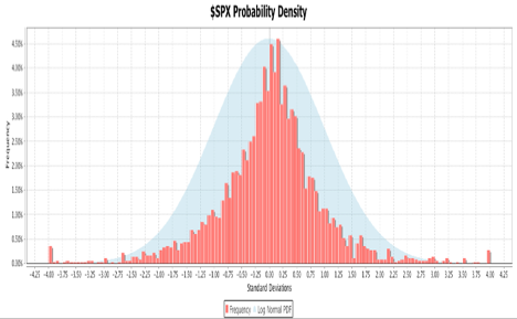
In the normal PDF exhibited above the tails of the distribution decline smoothly and approach zero as the number of standard deviations approach negative and positive infinity. In a fat tail PDF the extremes of the distribution are elevated to take into account periodic extreme moves in asset returns. The chart below is an example of an empirical, fat tail PDF for the S&P-500 index. The daily return data were collected for 10-year period ending in June of 2013. In the histogram the eight standard deviation range from -4.0 to +4.0 is divided into 128 buckets. The height of the bars indicates what percentage of the return data falls into each bucket. The histogram is superimposed over a normal distribution to illustrate the differences in the tails. From Equation 1, the number of standard deviations is calculated using Equation 3.
Equation 3
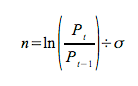
where:
Pt = The closing price for the current day
Pt-1 = The closing price for the previous day
σ = The standard deviation of the returns.
Each day’s closing price is compared to the previous day’s price to determine the return in terms of standard deviations. Each bucket encompasses a 0.0625 standard deviation range, the eight standard deviation total range divided by 128 buckets. To determine in which bucket a reading belongs, subtract the minimum value from the reading and divide by the bucket range. Changes greater than or equal to 4 standard deviations are counted in the highest bin. Changes of more than -4 standard deviations are placed in the lowest bin.
Tune in next time for Part 4 to see how to learn about the Empirical CDF. For powerful option trading software that calculates expected return, subscribe to Option Workbench.
![]()
© 2023 The Option Strategist | McMillan Analysis Corporation