
By Craig Hilsenrath
For the Introduction, an explanation of Expected Value, and Expected Value and Option Strategies refer to Enhancing Option Portfolio Returns Using Probability and Statistics - Part 1 & Part 2.
Determining the Probabilities
In 1973 Fisher Black and Myron Scholes published a paper defining the now famous Black-Scholes option pricing model. One of the characteristics of the Black-Scholes model is that it assumes that the underlying asset’s daily returns follow a log-normal distribution. The reason for this assumption is so that the model can estimate the probability that the option will expire in the money and earn a profit for the option buyer.
There are two concepts that need to be understood in order to comprehend how the probabilities are calculated. The first, the probability density function or PDF, is defined as a function that describes the relative likelihood for a random variable to take on a given value. The figure below shows a typical normal probability density function. The x-axis shows the change of the variable, the underlying price return in our case, in standard deviations. The Greek letter μ is used to represent the mean or average change.
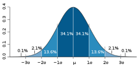
In the context of the Black-Scholes pricing model this means that the distribution of the natural logarithm of daily returns conforms roughly to the normal distribution. What the PDF tells us is the frequency at which we can expect the log return to change by a certain number of standard deviations. However, this is not the probability. As indicated in the diagram, the probability is represented by the area under the PDF. Taking the sum of the numbers representing the area between -3 and +3 standard deviations results in the 99.7% confidence interval.
To calculate the probabilities we need to know the area under the PDF curve for the number of standard deviations represented by the price change. This is accomplished by using the Cumulative Density Function or CDF. Figure 2 below shows the CDF for the normal distribution depicted in Figure 1.
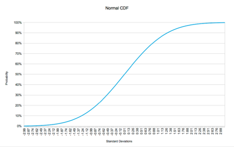
It is important to note that a point on the CDF designates the probability of the variable being less than or equal to the corresponding number of standard deviations. Therefore, the probability of the price moving zero or less standard deviations is 50%. Likewise, the probability of the price moving more than zero standard deviations is 50%.
How does this help us to derive the probabilities we need to calculate the expected profit? Another property of the CDF is that it can be used to calculate the probability of the variable falling between two points on the curve. This is accomplished by subtracting the probability at the lower end of the interval from the probability at the upper end of the interval. In mathematical terms:
Equation 2
F(xL < x ≤ xU) = F(xU) - F(xL)
Referring back to Table 1, the probabilities stated in the second column were actually determined by using the formula above and a $5 interval. So the 23.82% probability of the underlying being at $55 is actually the probability of the underlying being between $50 and $55. For that simple example a $5 interval was sufficient. However for actual trading a much smaller interval is needed.
Before deciding on what interval is appropriate there is a tradeoff that needs to be considered. In the example in Table 1 nine values for the underlying price were evaluated. In each step the probability, the value of the call, the theoretical profit and the probable profit were calculated. The probable profit for each row is the probability times the profit from the weighted average sum formula above. Computing the probability and the value of the call are both complex, multi-step calculations. As such, performing these calculations too many times can consume a great deal of computational resources.
Since a stock price cannot move less than one penny it may be tempting to pick a small interval around a penny. For example, the interval p - 0.005 < p ≤ p + 0.005 will yield a very precise probability. In the previous example the range from $31.94 to $78.28 will result in 4,634 prices to consider. If the volatility assumption is increased from 25% to 50% annualized the number of prices increases to 10,214. So changing the volatility assumption can make a big difference in the number of calculations that are performed. When contemplating the wide dispersion of possible underlying prices and the variety of volatility scenarios, it is easy to see that using the price-based interval can lead to vastly different consumption of computational resources.
As it turns out the differences in the probabilities using the $0.01 range are so minuscule that the extra computations are not worth the effort. A better solution that results in more than adequate results is to divide the range into equal size chunks. The objective is to choose a chunk size that results in a small enough difference in the probabilities without incurring undue computational expense.
Given that the endpoints of the price range are defined in terms of standard deviations, it makes sense to use an increment of standard deviations to divide the range. For example, using 1/128 of a standard deviation (a nice round computer number), divides the six standard deviation range into 768 chunks. Table 2 below shows a revision to the long call example above. A new column showing the number of standard deviations has been added. As the table shows this long call still has a positive expectation. If a trader could buy a call like this many times, on average, a profit of $76.34 per contract would be expected.
Tune in next time for Part 4 to learn about Fat-Tail Distributions. For powerful option trading software that calculates expected return, subscribe to Option Workbench.
![]()
© 2023 The Option Strategist | McMillan Analysis Corporation