
By Lawrence G. McMillan
This article was originally published in The Option Strategist Newsletter Volume 13, No. 3 on February 12, 2004.
One of the most tantalizing, yet dangerous, items in all of trading is the expensive option. From an elementary viewpoint, one would like to sell the option and collect the time value premium decay as it wastes away to nothing. But, more often than not, the options were expensive for a reason, so the option seller suddenly finds himself fighting the trend of a volatile movement by the underlying. In this article, we're going to discuss a few of the things to look for and then suggest a strategy that might be a "middle ground" where a skew is also involved with the expensive option (which it often is).
There are various ways that one might define an option as "expensive” our standard definition is that option's implied volatility is in the 90th percentile of past implied volatility readings (over the past 600 trading days, say, although one could use shorter time frames without changing the basic definition).
Expensive options appear with more frequency in stocks than in futures or indices. One would ordinarily expect stock options to have higher absolute implied volatilities, and they do since stocks are the most volatile one of the three. But when one considers the percentiles of implied volatility, there is no particular preponderance of occurrences amongst the three types of options - futures, stocks, or indices. Having said that, there are more occurrences of expensive stock options merely because there are more stocks with listed options than there are futures or indices. The following discussion will apply equally well to all options.
Naked Option Selling
The simplest strategy in dealing with expensive options is merely to sell them naked. This, of course, is quite risky and is a strategy that is not suitable for most people. In fact, even the most experienced professionals occasionally get burned by selling naked options.
The best way to avoid trouble when selling naked options is to sell index options when they are expensive. We have gone over a number of guidelines and rules for naked option selling in the past, but that is the most important rule. Indices don't gap; they don't get taken over; they don't report had earnings. They trade more or less in a continuous pattern. Moreover, indices are usually relatively high-priced so that the striking prices extend well away from the current index price – a feature that aids in follow-up action. Not only that, but the striking prices are closer together, percentagewise, than they are for lower-priced items such as stocks. This fact, too, aids in follow-up action.
Typically, a naked index option seller would sell both out-of-the-money calls and out-of-the-money puts (a naked strangle). The farther out-of-the-money the options are, the less chance there is of getting in trouble.
However, trouble can still occur – usually at the very worst times. This is why naked put sellers were decimated in the Crash of '87, for example. The market fell so fast and implied volatility inflated so rapidly that puts sold for a dollar were trading at horrendously large prices – over 100 in some cases. If one survives something like that once, he usually looks for another method of trading after that1. There have been many other, less extreme, times when naked option sellers were devastated by extreme market moves, too.
Option Spreads
Some traders figure that option spreads will hedge them and they will therefore not get wiped out as is possible with pure naked option selling. As it turns out, most of the time when one spreads expensive options he gives away nearly all of the statistical edge because he buys an expensive option to hedge the expensive option he sells. This is especially true in the case of the simplest spread – the credit spread, where one buys more deeply out-of-the-money options to hedge the outof- the-money options he sells. While I do acknowledge that credit spreads can be useful in lowering margin requirements (buy the out-of-the-money options very deeply out-of-themoney – expecting them to expire worthless, but taking advantage of the fact that the margin is the distance between the strikes in the spread, as opposed to the more onerous naked option margin).
Delta Neutral Option Selling
A more sophisticated approach is to sell the expensive options, and hedge them with either long options or a long position in the underlying. Generally, one uses the delta of the various instruments to create a delta neutral position initially. These positions generally fall into the category of a ratio write or a ratio spread. Naked options are still involved, so a large move can be very detrimental, but the ratio spread often pushes the breakeven point quite some distance away, which allows time for adjustment or closing the position if it begins to show signs of getting in trouble.
The typical ratio spread has a construction something like this:
  With XYZ at 68,
      Buy 5 XYZ July 70 calls
      and sell 8 XYZ July 80 calls
Initially, the spread is delta neutral, and is established for a small debit, or perhaps even money or a credit. The breakeven point – if this spread were established for even money – would be at 96.7, well above the current stock price of 68. Moreover, if the stock is near 80 at expiration, profits can be substantially larger than they would have been from merely selling naked July 80 calls.
Of course, above 96.7, there is large – virtually unlimited – risk and the spreader must pay close attention to his position, not letting it get too far above that price.
Volatility Skews and Expensive Options
The above descriptions of the strategies involving expensive options were rather general in nature, but now we want to get down to some specifics. It is often the case that expensive stock or futures options also involve a volatility skew. That is, the options at various striking prices have different implied volatilities – with the most expensive ones being either the farthest out of the money and/or the shortest-term options. The following table gives an example of how implied volatilities might be distributed in a stock that has either fallen dramatically or is perceived to have the ability to do so shortly.
              XYZ: 68:
         Implied Volatilities:
       Month: Mar  Apr  July  Oct
  Strike
   50         58%  55%  50%   45%
   60         54%  51%  47%   43%
   70         48%  45%  43%   42%
   80         43%  42%  41%   40%
In this example, if one were to sell the March 50's (with a 58% implied volatility) and buy, say, the July 70's (with a 43% implied volatility) he would have an attractive spread since the option he sold is statistically so much more expensive than the option he is buying. Of course, there is still risk and one would usually construct the spread between the two options in line with his risk appetite.
One ratio spread that we sometimes recommend is in the S&P futures options. It is most attractive when the out-of-the-money S&P puts (or $SPX, or $OEX puts) are quite expensive when compared with at-the-money puts - as they are now and usually have been since the Crash of '87. Such a spread is recommended this week in the "volatility skew" section on page 8.
That S&P spread involves deeply out-of-the-money naked index options, and as previously stated, index options have less risk. But it's stock (and sometimes futures) options that often seem the most attractive to sell, as they sometimes get very expensive. And that's where the dilemma arises. How can one sell these options – knowing full well that a large move is probably going to ensue. Yet, how can one buy them, either, in good conscience? Because if the big move doesn't develop, then a very large loss will result as the purchased options collapse under the dual weight of time decay and decreasing volatility.
This is an age-old problem that can be "attacked" in several ways. For example, we have previously written about a skew strategy in which one buy (expensive) straddles and tries to mitigate the possible loss that would occur if the underlying does not make a big move, by also buying calendar spreads – hoping that the calendar spread's profit will greatly reduce the straddle's loss if the stock doesn't move. The other possibility is that the stock does move a lot, and the straddles profit by more than the calendar spreads lose. As we concluded in The Option Strategist, Volume 12, No. 20, a ratio of about 3 long straddles and 10 calendar spreads is about "right" for such a strategy. Typically, it looks like this;
  With XYZ at 25 in February:
         Buy 10 May 25 calls
         Sell 7 March 25 calls
         Buy 3 March 25 puts
The main problem with such a strategy is that it can't be employed if the options are all relatively expensive to start with – for any decline in volatility will harm both the calendar and the straddle, overcoming the time decay benefits of the calendar. Unfortunately, when the options are all expensive, the strategist sometimes guesses whether to either simply buy the straddles or simply buy the calendar spreads – eschewing the companion strategy. The results from doing so can also generate losses if the "right" thing doesn't happen (albeit a limited loss).
Sometimes, though, another strategy can be employed when expensive options show a skew. As previously stated, a ratio spread is a viable strategy, but usually the skew is in the direction where the ratio spread could get into trouble. For example, if it's the out-of-themoney puts that are expensive, then one might be inclined to try to establish a put ratio spread. But that spread has downside risk and that's exactly why the out-of-the-money puts are so expensive – because there's a greater than normal chance that something bad is about to be announced.
The alternative strategy that is going to be described, though, can sometimes mitigate this. It's somewhat akin to legging into a ratio spread -- t only if you have to. Although we can't follow Will Rogers advice: "Only buy stocks that go up. If they don't go up, don't buy 'em," we can come close sometimes. This is one of those times.
In recent weeks, we have spotted expensive and skewed options in Nat Gas, Silver, and Gold. The skew was a positive one, in that the expensive options were the out-ofthe- money calls. In each case we used a bull spread to approach the trade, rather than using a call ratio spread. Why? Because we didn't want to risk being short naked calls in a strongly rising market. Note that a bull spread still benefits from the skew, as the option you're buying (an at-the- money call, say) has a lower implied volatility than the out-of- the-money call you're selling. In the case of Nat Gas, the market went straight up and we maxed out the bull spread. In gold, the market went up for a while, and we took partial profits, but then it slipped and we were stopped out of the final portion. In the Silver spread, however, a third scenario developed: Silver dropped below technical support, and we then converted the bull spread into a ratio spread because at that point, we felt there was less risk of an upside blowout and a neutral stance could be beneficial.
Let's examine the strategy to see how this might apply. We will use the Silver call bull spread in this example, but understand that the principle works equally well for any stock, index, or futures skew where the out-of-the-money calls are the expensive option – and it works well, too, for put bear spreads where out-of-the-money puts are the expensive option.
Here is how the Silver situation looked initially:
May Silver futures: 636
  Call     Price  IV    Delta
  May 630   42    30%   0.56
  May 650   35    32%   0.48
  May 670   28    34%   0.41
  May 680   25    35%   0.37
An attractive skew exists between the May 630 calls (which
would be bought) and the May 680 calls (which would be
sold). If one were to establish a delta neutral position, he'd
buy 2 and sell 3 (the ratio of the deltas – 0.56 to 0.37 – is 3
to 2), which would entail a debit of 9 points ($450).
However, that spread would have upside risk above 770.
Since Silver was in such a strong uptrend at the time, we decided to use a simple call bull spread instead – buying the May 630 calls and selling an equal number of May 680 calls – a strategy which still benefits from the skew between the two calls. One bull spread incurs a debit of 17 points ($850). We don't really want to risk the entire $850, but if the futures rise in price, we don't mind incurring that debit to make a potential profit of $1650 – which would occur if the futures were above 680 at expiration. This is all quite simple up to this point, but you might be wondering where does the Will Rogers analogy come in? Where do I have a chance to erase that debit if things go awry and Silver futures fall instead?
The answer is that if the underlying falls and breaks support, we can simply convert the position into a ratio spread at that time. While the prices may not be as attractive as they initially were, such an adjustment can be made after the upside momentum of the underlying has been broken. Hence, later, when May Silver futures fell below support at 610, we sold enough of the May 680 calls to produce a delta neutral spread (see Position F260 on page 5). Now, it's still possible that May Silver futures could rise again and still get us into trouble on the upside before the April 27th expiration date, but the longer it takes before such an adjustment needs to be made, the less likely there is to be an upside problem.
Let's forget what actually happened and instead look at the theoretical possibilities of such a spread. We'll use stock options to make the calculations easier (at $100 per point). Suppose that one bought five April 60 calls and sold 5 April 70 calls, initially for a debit of 1.0 each ($500 total debit, plus commission). Also, suppose that's more than we really want to risk on this trade. At first, we will see if the underlying rises in price; if it does, we will profit without having to worry about naked options.
But if the underlying doesn't rise, or begins to fall, then we can sell out some of the long April 60 calls to create a ratio spread, after the fact. As a simple example, suppose you are willing to risk $100 on this trade - not the original $500 debit incurred. You could just wait until the spread shrunk by 20 cents – which is $100 on five spreads – and stop yourself out. But that might happen very quickly, stopping you out before your spread has a chance to work.
Alternatively, if the underlying stock begins to fall, you could sell out some of the long calls, recovering enough credit to get your risk down to the level you desire. In this particular case, one wants to recover $400 from the sale of April 60 calls (that he owns) in order to reduce his debit from $500 to $100 – the level that he wants to risk if the underlying declines and all the calls expire worthless.
If he waits until near expiration to do this, then he needs to ensure that he receives at least 0.80 points for the five calls (that's $400). Since he paid 1.0 for the spread, this is the same 20-cent risk that we talked about earlier. So, if expiration is nigh, and the stock is falling from a higher price and drops to about 60.8, one could simply sell out the longs for 80 cents each, and remain naked the April 70 calls for a few days until expiration, and he would have lost only $100.
However, at times before expiration, he would not want to sell out all five calls for that would leave him naked the 5 Apr 70 calls that he is short. So, suppose that if the stock declines, he wants to sell only three of the five calls he is long. That means those three calls will have to bring in $400, or that he must sell them for roughly 1.35 points.
Here's what the position would look like in that case, after the adjustment:
  Long 2 April 60 calls
  Short 5 April 70 calls
  Debit incurred: $100
Such a spread has the profit graph shown below. It could make as much as $1900 if the stock were exactly at 70 at expiration. There is some risk below 60 at expiration, but the maximum risk is $100 (anywhere below 60 at expiration). The main problem is that there are large possible losses above 76.3 at expiration, but if one isn't forced to make the adjustment too soon in the life of the spread, the probability that the stock will rise to 76.3 in the remaining time will be small.
Where will XYZ stock have to be, and when for the Apr 60 calls to be selling at a price of 1.35? The following table answers that question, assuming that the calls retain their initial implied volatility of 30%:
  Time Remaining     Stock price at
  Until Expiration  which Apr 60 call
                    is worth 1.35 points
       75 days           55.5
       60 days           56.5
       45 days           57.5
       30 days           58.7
       15 days           59.6
So, if the stock falls to the price in the right-hand column with the days remaining in the left-hand column, the spreader would convert his bull spread into a ratio spread at that time. Obviously, the stock would be heading downward when that happened, and the amount of time left for it to rally back to 76.3 (the upside breakeven) would be lessened. Both of those facts lessen the upside risk as a probability. This gives you a lot more leeway than stopping yourself out for a 20 cent loss in the initial bull spread.
Summary
So, when you spot a skewed situation, see if the bull (or bear spread) is viable. Does the chart support a directional position initially? If so, that may be the better tack - not risking a naked option position initially. Then, later, if the underlying moves the "wrong" way, a ratio spread can be established – still taking advantage of the skew.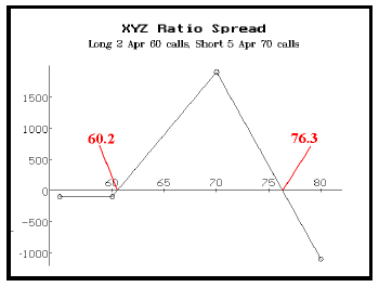
This article was originally published in The Option Strategist Newsletter Volume 13, No. 3 on February 12, 2004.
© 2023 The Option Strategist | McMillan Analysis Corporation