By Lawrence G. McMillan
This article was originally published in The Option Strategist Newsletter Volume 14, No. 6 on March 25, 2005.
In a press release issued on March 18th, the CBOE has announced that option trading on $VIX will begin on Friday, April 22 (2005). We consider this to be a major new derivatives product. It is the first time that there will be the opportunity to trade options on volatility in a listed marketplace (they have traded over-the-counter, institutionally, for some time). In today’s article, we’ll not only look at the mechanics of these options, but at some of the theory as well.
This product will be useful for a wide range of applications for stock and option traders. Wherever $VIX futures were applicable, these options will be as well. Furthermore, option strategies on $VIX can now be constructed – with their own unique sets of risk and reward parameters. As we will discuss in this article, however, $VIX does not behave like a stock, so there will have to be some adjustments for that fact in the modeling of $VIX option prices.
The Basics
These are cash-based index options, similar to $SPX or $OEX or $DJX options or any other index option. The underlying contract is the $VIX cash index itself, not the $VIX futures contract that trades on the CBOE Futures Exchange (CFE). Thus, it is not necessary for one to have a futures account in order to trade these $VIX options. However, we would certainly encourage all traders who plan on using these new options to open a futures account so that $VIX futures can be employed as a hedge, if need be.
A similar companion set-up was used for years by most astute traders in $SPX and $OEX options; they had a futures account for trading S&P 500 futures against positions in those CBOE-listed options. Eventually SPDRs (SPY) came along and allowed one to hedge $SPX option positions directly. But there is no ETF or SPDR for $VIX, and probably won’t be, so if any hedging strategies are to be employed, it will be necessary to have a futures account in which the $VIX futures can be utilized.
Some of the nomenclature and specifications of the futures contract are going to be used for these new, listed $VIX options. $VXB is an index that is $VIX times 10. This is to be the underlying index for these new $VIX options. And, in fact, the options will have a base ticker symbol of VXB. Striking prices will be at least 2-1/2 points apart, so this might be a typical array of strikes at a given time:
$VIX: 14.24
$VXB: 142.40
Strikes available for VXB options: 130, 132.5, 135, 137.5, 140, 142.5, 145, 147.5, 150, etc.
The options will be traded and quoted as $100 per point, as are all listed options, so if a VXB Dec 150 call is selling for 9, that means it will cost $900 for one contract.
Also, similar to the futures, these options will have their last trading day on Tuesday prior to the third Friday of the expiration month. The settlement day for these options is an “a.m.” (Morning) settlement on the Wednesday prior to the 3rd Friday of the expiration month. These are exactly the same days that the futures expire and settle. Continuing this similarity, the actual settlement value of the cash-based options will be based on a “special opening quotation (SOQ)” derived from the opening trades (or if no trade, then the average opening bid and offer) of the options used to calculate the $VIX Index itself.
These options will trade until 4:15pm Eastern time each day, as do $SPX and $OEX options. At any one time, four series will be listed – the same four expiration as the $VIX futures, in fact: the two near-term months, plus the next two months in the February cycle (i.e., Feb, May, Aug, Nov).
Pricing Considerations
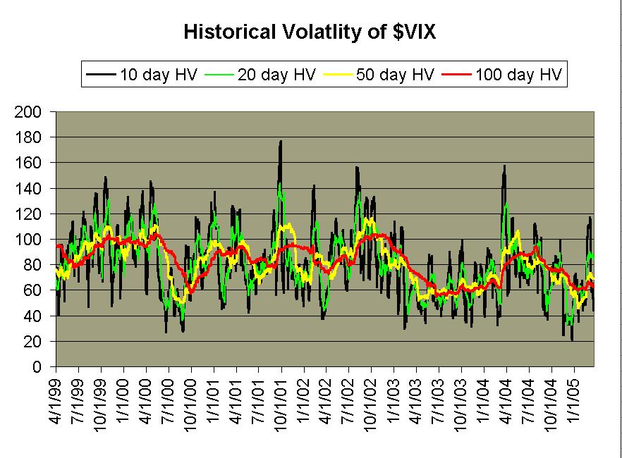
In order to price $VIX options, we first need an estimate of the volatility of $VIX – i.e., the volatility of volatility. While that may sound a bit strange, it’s exactly what needs to be measured in order to estimate the price of an option on volatility. The above graph shows the historical volatility of $VIX over the past six years. This time frame encompasses the end of the previous bull market, plus the ensuing bear market, and now the rally since March, 2003. In other words, various market conditions are present in this graph. Moreover, the actual price of $VIX has varied greatly over that time. It rose to 60 or so in the bear market, and then collapsed to nearly 10 in the last year. Once again, a great variance in the price of $VIX is encompassed in the above data. However, the one thing that stands out is that – bull market or bear, high-priced $VIX or low-priced – the historical volatility of $VIX remains amazingly constant: averaging about 80%.
The red line on the chart is the 100-day historical volatility and it has generally ranged between 60% and March 25, 2005 There is risk of loss in all trading Page 3 Figure 2 Figure 3 100%. The green line is the 20-day historical – often the time frame of choice used by traders for a volatility estimate – and it has ranged between 40% and 120% (again, with 80% being the middle of that range).
The black line is the 10-day historical and it has, of course, had the most extreme readings. The highest spikes on the chart occurred at times of significantly high $VIX reandings (and hence, at major market bottoms): September 2001, July 2002, and March 2003.
For a moment, let’s assume that the Black-Scholes model can be used to value these options (it sometimes can’t, as will be shown shortly). Using an 80% volatility estimate, VXB options would be theoretically priced as follows:
Example: assume $VIX is at 14, and thus VXB is at 140. The following option prices on VXB might theoretically exist. Furthermore assume that these are being priced one month before May expiration
VXB: 140
VXB Theoretical Option Prices
| Month/Strike | Call | Put |
| May 130 | 18.30 | 8.00 |
| May 140 | 13.10 | 12.90 |
| May 150 | 9.10 | 18.90 |
The problem with using the Black-Scholes model for valuing $VIX options is that $VIX does not conform to a lognormal distribution. For example, we know that there is a “floor” and a “ceiling” on $VIX. While these limits are not fixed ($VIX could theoretically trade down to 5, say, although it has never happened; or $VIX could trade up to 100, although that has never happened either).
Restated: when $VIX is near 10, there is a much larger chance that it will rise than fall. Or if it’s near its all-time highs in the 40's, there is a much larger chance that it will fall than rise (note: if you recall $VIX shooting up to 60 in 2002, you’re not losing your memory – but $VIX is not computed the same way now as it was then; what we now call $VXO had those higher readings). Neither of those descriptions fits a lognormal distribution. Moreover, it appears that $VIX conforms to different distributions, depending on where it’s trading at the time.
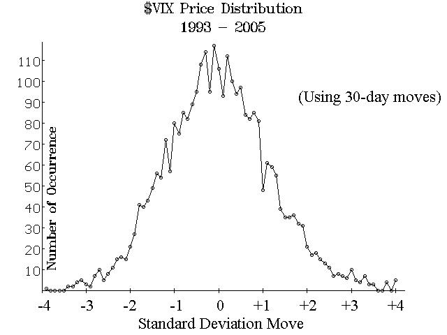
Figure 2 shows the 30-day movements, expressed as standard deviation moves, of $VIX from 3/1/93 through 3/21/05. There are slightly more than 3000 such data points, comprising this graph. If prices are lognormally distributed, then this graph should resemble a true Bell curve. In fact, it does resemble a Bell curve. It’s not exactly a Bell Curve, though: since about 1500 times there were negative movements, but 1400 times showed positive movements ($VIX being unchanged in the other 100 samples).
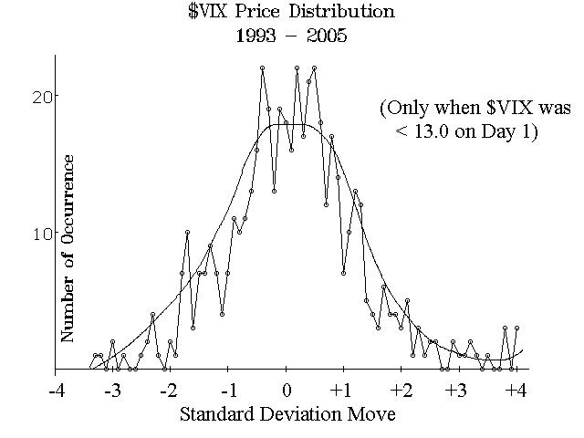
Figure 3 is a further refinement of the data. In this graph, only cases where $VIX was trading at 13 or less on Day 1 were considered. Otherwise, it is the same sort of data shown in Figure 2: 30-day moves, converted to standard deviations. Notice that when $VIX is that low to begin with, there were no moves of -3.5 standard deviations or more. Furthermore, this one doesn’t even really resemble a Bell Curve. There are about 230 points in which $VIX had a negative move after 30 days, and 260 in which it had a positive move. Hence, this distribution – as expected – shows a greater tendency for $VIX to rise than fall, when $VIX is initially low to begin with.
Without showing another graph, we ran a similar study to see what the $VIX movements occurred when $VIX began at a price of 35 or higher. There have only been 96 such days since 1993. Of those 96, 58 times $VIX moved lower over the next 30 days, while it moved higher only 38 times. This is what we expected, of course – that $VIX has a sort of “cap” on it at higher prices and hence has a tendency to move lower in these cases. By inference, if we throw out the “extreme” points, then $VIX does more or less conform to a lognormal distribution. Hence – despite the problems near the extremes – we can say that most of the time $VIX movements seem to be lognormally distributed. This is helpful, for it means that if $VIX is not near the extremes, then perhaps the Black-Scholes model can indeed be used to value $VIX (actually, VXB) options.
However, when $VIX is near the extremes, if one is using a Black-Scholes model to value the options, he will see a steep skew. The skew will be positive (or forward) when $VIX is low. That is, outof- the-money calls will seem expensive with respect to out-of-the-money puts. Conversely, when $VIX is very high, then a negative (or reverse) skew will be evident: out-of-the-money puts will be trading with a higher implied volatility than out-of-the-money calls. If one understands these limitations, then I believe the Black-Scholes model can be used for valuing these new $VIX options. In actual practice, we will see how these valuations play out.
This article was originally published in The Option Strategist Newsletter Volume 14, No. 6 on March 25, 2005.
© 2023 The Option Strategist | McMillan Analysis Corporation