By Lawrence G. McMillan
This article was originally published in The Option Strategist Newsletter Volume 19, No. 18 on October 1, 2010.
Most of the time, we look at index options in order to make general observations about volatility. These observations, which evolve into opinions, often involve $VIX, $VIX futures, or $VIX options, all of which are based on the $SPX options. This is a reasonable approach, of course, since $SPX options are heavily traded, as are the $VIX derivatives, and therefore they reflect the greed, fear, and anticipations of literally millions of traders.
However, index options may also react in extreme ways at times, and that can present a somewhat incorrect – or at least, distorted – view of implied volatility. In such times, it can often be useful to look at stock options to see if a different volatility picture emerges. This is one of those times. Simply stated, the average stock’s options are currently in a very low percentile of implied volatility – in the low teens. Conversely, we know that index options are quite expensive by a) the relatively high level of $VIX and b) the extreme steepness of the term structure of the $VIX futures. What is causing this apparent discrepancy, and can we take advantage of it? Yes, we can. Let’s see how.
Let’s first concentrate on the equity options. When we say that the average stock’s options are in a certain “percentile of implied volatility,” we look back 600 trading days to make that determination. A specific example might help to quantify this process:
Example: IBM is trading near 135.
Each day, we calculate a “composite implied volatility1” (CIV) for IBM, and for every other entity that trades listed options (there are about 5,000 in all – counting futures, indices, ETF’s, and stocks).
This CIV is determined by taking each individual IBM option’s implied volatility and weighting each one by its trading volume and distance in-/out-of-the-money (at-the-money gets the most weight). This weighting then produces one single number each day that is representative of the implied volatility level of IBM options: the “composite implied volatility.”
Today, in IBM’s case, the CIV is 17.1%. Comparing 17.1% with the IBM CIV’s of the past 600 trading days, we see that this current reading is in the 13th percentile. That is, in the last 600 trading days, there were lower daily CIV’s only 13% of the time; 87% of the time the CIV was higher. Thus, based on the history of implied volatility, these IBM options are relatively cheap.
In each issue of The Option Strategist, we publish a graph of the distribution of CIV’s for all stocks. This graph is usually on page 8, as it is in this issue. The graph also denotes the average stock’s CIV percentile.
At the current time, the average CIV percentile has dropped to extremely low levels, with readings of 11%, 12%, and 13% having occurred in the past week. This describes a market with quite cheap equity options. Of course, they could get even cheaper, but one should begin planning now for what this cheapness implies.
What kind of information can we glean from the CIV? The graph below, in Figure 1, shows a historic graph of the daily average CIV of all stocks, plotted against the $SPX Index. Broad market buy signals are marked on this graph, by vertical red lines.
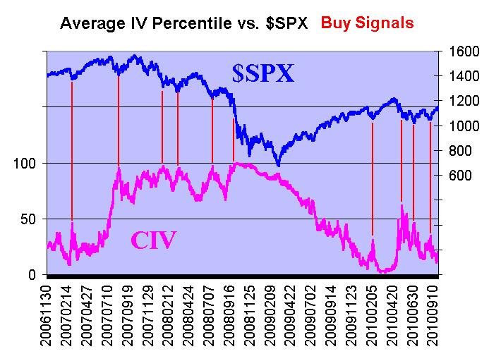
We placed these buy signals (red lines) at local maxima (i.e., peaks) on the graph. Except for the October, 2008, signal (where the CIV was “mashed” up against the top of its graph – at the maximum, 100 level, for weeks on end), these were good intermediate-term buy points for $SPX.
Of course, we have seen similar things from the chart of $VIX, where we know that spike peaks in $VIX during a declining market are intermediate-term buy signals. So, this isn’t really any “new” information; it’s just the same information presented in a slightly different format. To see that more clearly, consider Figure 2.
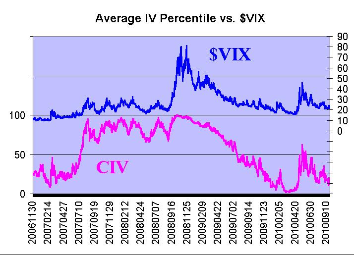
The patterns of CIV and $VIX are very similar. Of course, $VIX – which didn’t have a cap on it at 100 – rose much higher in the 2008 debacle, but other than that the two are very comparable graphs.
Perhaps more interesting, though, is what happens when CIV gets “too low.” Figure 3 shows the same two graphs as Figure 1, but this time we’ve marked sell signals on them, using “troughs” in CIV as the actual sell point.
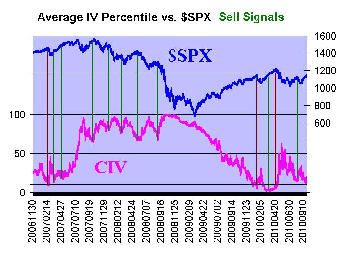
The green lines denote sell signals that emanated from almost anywhere on the chart. They have a relatively good track record, but there are some poor ones such as March and April, 2007, and March, 2010.
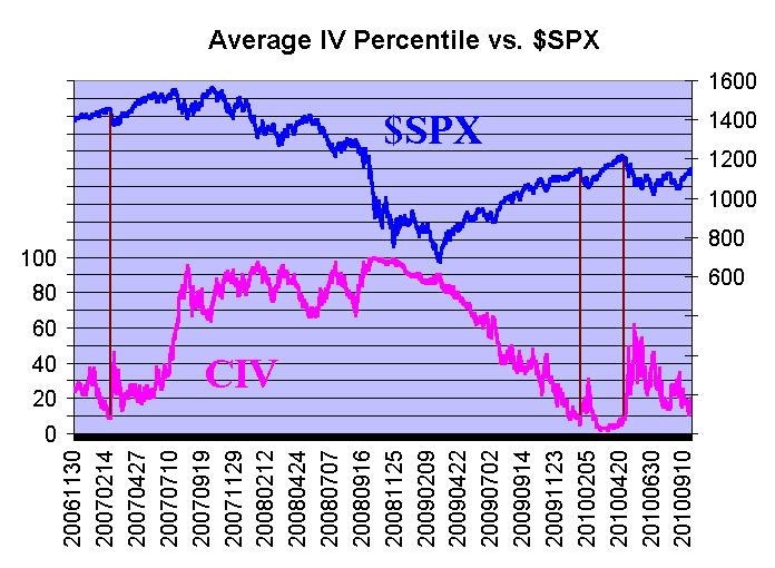
But if we refine the data in Figure 3 a bit and only concentrate on the sell signals that came from very low levels, then they are much more successful, although there are only a few of them. The brown vertical lines denote sell signals than arose after CIV had declined to 10 or lower. This is more clearly shown in Figure 4, where the brown lines are the only sell signals. The rule of thumb here is that once CIV falls to 10 or lower, then sell $SPX when CIV rises back to 15 or higher.
This has only resulted in three signals since 2006: 1) in February, 2007, a sell signal was given shortly before the markets broke down badly when China constricted speculative margin; there was also a “$VIX below 10" sell signal in effect at that time; 2) in late January, 2010, shortly before $SPX sold off about 100 points; and 3) in late April, 2010, shortly before $SPX sold off 180 points, including the May “flash crash.”
So, only a few sell signals, but very good ones. What makes this relevant, of course, is the fact that we are now flirting with another sell signal. CIV fell as low as 11 last week – and if you’re a stickler for details, then you might say it hasn’t reached 10 yet. But if you look at the bigger picture, you can see that stock options have gotten “too cheap” again, and that generally is a negative warning sign for the stock market. And this time, $VIX seems determined to stay in the 20's, so this might be the only “low volatility warning” that you get.
Index Options vs. Equity Options
Currently, there seems to be a massive dislocation between equity and index options. $VIX is relatively high (near 22), and $VIX futures have a very steep term structure on top of that. These, of course, are as a result of the prices of $SPX Index options. So index options appear to be rather expensive, but stock options are “cheap.” What is going on here?
The answer lies in the “skew” of the options. It is almost always true that – for index options – out-of-themoney puts are quite expensive with respect to at-themoney puts; conversely, out-of-the-money call options are cheap with respect to at-the-money calls. We publish a table of $OEX implied volatility skews each week (usually on page 8, as it is today). By the way, these skew properties pertain to ETF options on broad-based indices as well.
Since this pattern pertains mostly to different strikes, and not different months, it is called a “linear skew” by many traders. Furthermore, since the lower strikes are more expensive, it is called a “reverse skew” or “negative skew.” Currently, this skew exists in many stock options as well, as traders are buying out-of-the-money puts as protection against a market decline.
This contrasts with the recent upside breakout and generally lower volatility of a bullish market trend, where option premiums are lower, in general. So the CIV is low because it weights at-the-money options most heavily, but $VIX and its derivatives are higher because they consider the weighting of heavily-traded, out-of-the-money puts. Let’s look at a simple example, using SPY and IBM options, where the reverse skew is evident in both.
Example:
| SPY: 114.67 | IBM: 135 | ||
| Option | Implied | Option | Implied |
| Oct 102 put | 30% | Nov 110 put | 28% |
| Oct 108 put | 24% | Nov 120 put | 23% |
| Oct 114 put/call | 20% | Nov 130 put | 19% |
| Oct 116 call | 18% | Nov 135 put/call | 18% |
| Oct 118 call | 17% | Nov 140 call | 17% |
| Oct 120 call | 16% | Nov 150 call | 16.5% |
It should be noted that, as long as arbitrage is available (i.e., the stock can easily be borrowed for selling short by arbitrageurs), a put and call at the same strike will have essentially the same implied volatility.
Strategy
When a reverse skew exists, a volatility trader wants to sell the lower strikes and buy the higher strikes. In doing so, he is selling the options with higher implied volatilities and buying those with lower implieds.
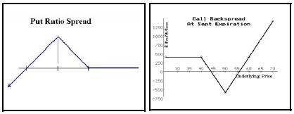
The strategies that lend themselves to this approach are 1) bear spreads with puts or calls, 2) put ratio spreads, and 3) call backspreads. Of these three strategies, the bear spread is the most directional. If one establishes that, and the market rises, he will lose money.
The other two, though, allow one a chance to profit under several sets of circumstances. The put ratio spread – assuming it is established for a credit – will make money as long as the market doesn’t fall too far, too fast. It is often best established when options are expensive.
The call backspread, on the other hand, is usually the method of choice when options are expensive. It can make a profit if the market rises sharply, but it can also make a (limited) profit if the market falls sharply. The graphs at the top of the next column show the general shape of the profit graph of the put ratio spread and the call backspread.
Before getting into specifics, there is one other piece of background information that you’ll need: a call backspread is equivalent to “a straddle purchase plus the sale of an out-of-the-money put.” This was described in a previous issue: Volume 17, No. 14. We call this version the “synthetic call backspread.”
We recently established one of these positions in Apple (AAPL) as Position E851. With AAPL at 252, we bought the Jan 260 straddle and sold the (more expensive) Jan 220 puts. AAPL quickly moved up to 288 last week, and – on the weekly Hotline update – we recommended closing out the position for a nice profit.
This type of position is warranted at the current time, in our opinion, because of the market and volatility conditions (cheap options with a reverse skew) described above. Many stocks have these parameters in place, but we want the ones with the best chance to make a move, and we want the steepest skew.
These positions can make money in either direction (although, they make more if the stock moves up). Since there is a reasonably good chance the market will move sharply lower, we want to be sure to allow for a large enough return in that case. In the synthetic straddle, the maximum downside profit is the difference in the strikes minus the straddle price. The larger that is, as a percent of the straddle price, the more downside profit room there is.
Summary
When options are cheap and skewed, the (synthetic) call backspread strategy is attractive – both from theoretical and practical standpoints.
This article was originally published in The Option Strategist Newsletter Volume 19, No. 18 on October 1, 2010.
© 2023 The Option Strategist | McMillan Analysis Corporation